Getting Started

This tutorial covers the most common type of experiment in reinforcement learning: the control experiment. An agent is supposed to find a good policy while interacting with the domain.

Note

If you don’t use the developer verion of rlpy but installed the toolbox via pip you can get the example scripts referenced in this tutorial as follows: Download the latest RLPy package from https://pypi.python.org/pypi/rlpy and extract the examples folder from the archive. In this folder you find several examples of how to use RLPy.

First Run

Begin by looking at the file examples/tutorial/gridworld.py:

#!/usr/bin/env python
"""
Getting Started Tutorial for RLPy
=================================

This file contains a very basic example of a RL experiment:
A simple Grid-World.
"""
__author__ = "Robert H. Klein"
from rlpy.Domains import GridWorld
from rlpy.Agents import Q_Learning
from rlpy.Representations import Tabular
from rlpy.Policies import eGreedy
from rlpy.Experiments import Experiment
import os


def make_experiment(exp_id=1, path="./Results/Tutorial/gridworld-qlearning"):
    """
    Each file specifying an experimental setup should contain a
    make_experiment function which returns an instance of the Experiment
    class with everything set up.

    @param id: number used to seed the random number generators
    @param path: output directory where logs and results are stored
    """
    opt = {}
    opt["exp_id"] = exp_id
    opt["path"] = path

    # Domain:
    maze = os.path.join(GridWorld.default_map_dir, '4x5.txt')
    domain = GridWorld(maze, noise=0.3)
    opt["domain"] = domain

    # Representation
    representation = Tabular(domain, discretization=20)

    # Policy
    policy = eGreedy(representation, epsilon=0.2)

    # Agent
    opt["agent"] = Q_Learning(representation=representation, policy=policy,
                       discount_factor=domain.discount_factor,
                       initial_learn_rate=0.1,
                       learn_rate_decay_mode="boyan", boyan_N0=100,
                       lambda_=0.)
    opt["checks_per_policy"] = 100
    opt["max_steps"] = 2000
    opt["num_policy_checks"] = 10
    experiment = Experiment(**opt)
    return experiment

if __name__ == '__main__':
    experiment = make_experiment(1)
    experiment.run(visualize_steps=False,  # should each learning step be shown?
                   visualize_learning=True,  # show policy / value function?
                   visualize_performance=1)  # show performance runs?
    experiment.plot()
    experiment.save()

The file is an example for a reinforcement learning experiment. The main components of such an experiment are the domain, GridWorld in this case, the agent (Q_Learning), which uses the policy eGreedy and the value function representation Tabular. The experiment Experiment is in charge of the execution of the experiment by handling the interaction between the agent and the domain as well as storing the results on disk (see also Overview).

The function make_experiment gets an id, which specifies the random seeds and a path where the results are stored. It returns an instance of an Experiment which is ready to run. In line 53, such an experiment is created and then executed in line 54 by calling its run method. The three parameters of run control the graphical output. The result are plotted in line 57 and subsequently stored in line 58.

You can run the file by executing it with the ipython shell from the rlpy root directory:

ipython examples/tutorial/gridworld.py

Tip

We recommend using the IPython shell. Compared to the standard interpreter it provides color output and better help functions. It is more comportable to work with in general. See the Ipython homepage for details.

Note

If you want to use the standard python shell make sure the rlpy root directory is in the python seach path for modules. You can for example use:

PYTHONPATH=. python examples/tutorial/gridworld.py

Tip

You can also use the IPython shell interactively and then run the script from within the shell. To do this, first start the interactive python shell with:

ipython

and then inside the ipython shell execute:

%run examples/tutorial/gridworld.py

This will not terminate the interpreter after running the file and allows you to inspect the objects interactively afterwards (you can exit the shell with CTRL + D).

What Happens During a Control Experiment

During an experiment, the agent performs a series of episodes, each of which consists of a series of steps. Over the course of its lifetime, the agent performs a total of max_steps learning steps, each of which consists of:

1. The agent choses an action given its (exploration) policy
2. The domain transitions to a new state
3. The agent observes the old and new state of the domain as well as the reward for this transition and improves its policy based on this new information

To track the performance of the agent, the quality of its current policy is assessed num_policy_checks times during the experiment at uniformly spaced intervals (and one more time right at the beginning). At each policy check, the agent is allowed to interact with the domain in what are called performance runs, with checks_per_policy runs occuring in each. (Using these multiple samples helps smooth the resulting performanace.) During performance runs, the agent does not do any exploration but always chooses actions optimal with respect to its value function. Thus, each step in a performance run consists of:

1. The agent choses an action it thinks is optimal (e.g. greedy w.r.t. its value function estimate)
2. The domain transitions to a new state

Note

No learning happens during performance runs. The total return for each episode of performance runs is averaged to obtain a quality measure of the agent’s policy.

Graphical Output

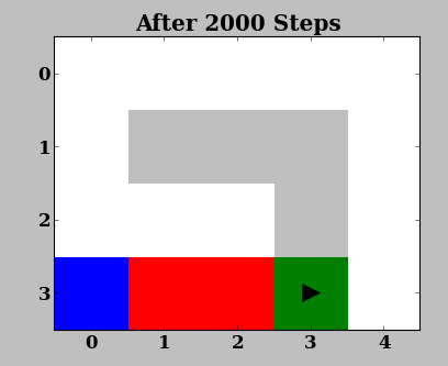
While running the experiment you should see two windows, one showing the domain:

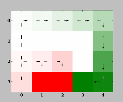
and one showing the value function:

The Domain window is a visual representation of the domain (here, GridWorld) and is useful in quickly judging or demonstrating the performance of an agent. In this domain, the agent (triangle) has to move from the start (blue) to the goal (green) location in the shortest distance possible, while avoiding the pits (red). The agent receives -0.001 reward every step. When it reaches the goal or a pit, it obtains rewards of +1.0 or and the episode is terminated.

The value function window shows the value function and the resulting policy. It is shown because visualize_learning=True. Notice how the policy gradually converges to the optimal, direct route which avoids pits. After successive iterations, the agent learns the high (green) value of being in states that lie along the optimal path, even though they offer no immediate reward. It also learns the low (red) value of unimportant / undesirable states.

The set of possible actions in each grid is highlighted by arrows, where the size of arrows correspond to the state-action value function \(Q(s,a)\). The best action is shown in black. If the agent has not learned the optimal policy in some grid cells, it has not explored enough to learn the correct action. (This often happens in Row 2, Column 1 of this example, where the correct action is left.) The agent likely still performs well though, since such states do not lie along the optimal route from the initial state s0; they are only rarely reached either because of \(\epsilon\)-greedy policy which choses random actions with probability \(\epsilon=0.2\), or noise in the domain which takes a random action despite the one commanded.

Most domains in RLPy have a visualization like GridWorld and often also a graphical presentation of the policy or value function.

At the end of the experiment another window called Performance pops up and shows a plot of the average return during each policy assessment.

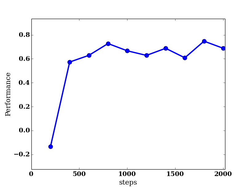
As we can see the agent learns after about 500 steps to obtain on average a reward of 0.7. The theoretically optimal reward for a single run is 0.99. However, the noise in the domain causes the agent to take the commanded action only 70% of the time (see the domain initialization in line 32); thus the total reward is correspondingly lower on average. In fact, the policy learned by the agent after 500 steps is the optimal one.

Console Outputs

During execution of examples/tutorial/gridworld.py, you should see in the console window output similar to the following:

647: E[0:00:01]-R[0:00:15]: Return=+0.97, Steps=33, Features = 20
1000 >>> E[0:00:04]-R[0:00:37]: Return=+0.99, Steps=11, Features = 20
1810: E[0:00:05]-R[0:00:23]: Return=+0.98, Steps=19, Features = 20

Each part has a specific meaning:

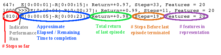
Lines with >>> are the averaged results of a policy assessment. Results of policy assessments are always shown. The outcome of learning episodes is shown only every second. You might therefore see no output for learning episodes if your computer is fast enough to do all learning steps between two policy assessments in less than one second.

Note

Throughout these experiments, if you see error messages similar to: rlpy/Tools/transformations.py:1886: UserWarning: failed to import module _transformations you may safely ignore them. They merely reflect that configuration does not support all features of rlpy.

A Slightly More Challenging Domain: Inverted Pole Balancing

We will now look at how to run experiments in batch and how to analyze and compare the performance of different methods on the same task. To this end, we compare different value function representations on the Cart-Pole Balancing task with an infinite track. The task is to keep a pole balanced upright. The pole is mounted on a cart which we can either push to the left or right.

The experimental setup is specified in examples/tutorial/infTrackCartPole_tabular.py with a tabular representation and in examples/tutorial/infTrackCartPole_rbfs.py with radial basis functions (RBFs). The content of infTrackCartPole_rbfs.py is

"""
Cart-pole balancing with randomly positioned radial basis functions
"""
from rlpy.Domains import InfCartPoleBalance
from rlpy.Agents import Q_Learning
from rlpy.Representations import *
from rlpy.Policies import eGreedy
from rlpy.Experiments import Experiment
import numpy as np
from hyperopt import hp

param_space = {
    "num_rbfs": hp.qloguniform("num_rbfs", np.log(1e1), np.log(1e4), 1),
    'resolution': hp.quniform("resolution", 3, 30, 1),
    'lambda_': hp.uniform("lambda_", 0., 1.),
    'boyan_N0': hp.loguniform("boyan_N0", np.log(1e1), np.log(1e5)),
    'initial_learn_rate': hp.loguniform("initial_learn_rate", np.log(5e-2), np.log(1))}


def make_experiment(
        exp_id=1, path="./Results/Temp/{domain}/{agent}/{representation}/",
        boyan_N0=753,
        initial_learn_rate=.7,
        resolution=25.,
        num_rbfs=206.,
        lambda_=0.75):
    opt = {}
    opt["exp_id"] = exp_id
    opt["path"] = path
    opt["max_steps"] = 5000
    opt["num_policy_checks"] = 10
    opt["checks_per_policy"] = 10

    domain = InfCartPoleBalance(episodeCap=1000)
    opt["domain"] = domain
    representation = RBF(domain, num_rbfs=int(num_rbfs),
                         resolution_max=resolution, resolution_min=resolution,
                         const_feature=False, normalize=True, seed=exp_id)
    policy = eGreedy(representation, epsilon=0.1)
    opt["agent"] = Q_Learning(
        policy, representation, discount_factor=domain.discount_factor,
        lambda_=lambda_, initial_learn_rate=initial_learn_rate,
        learn_rate_decay_mode="boyan", boyan_N0=boyan_N0)
    experiment = Experiment(**opt)
    return experiment

if __name__ == '__main__':
    experiment = make_experiment(1)
    experiment.run_from_commandline()
    experiment.plot()

Again, as the first GridWorld example, the main content of the file is a make_experiment function which takes an id, a path and some more optional parameters and returns an Experiment.Experiment instance. This is the standard format of an RLPy experiment description and will allow us to run it in parallel on several cores on one computer or even on a computing cluster with numerous machines.

The content of infTrackCartPole_tabular.py is very similar but differs in the definition of the representation parameter of the agent. Compared to our first example, the experiment is now executed by calling its Experiments.Experiment.run_from_commandline() method. This is a wrapper around Experiments.Experiment.run() and allows to specify the options for visualization during the execution with command line arguments. You can for example run:

ipython examples/tutorial/infTrackCartPole_tabular.py -- -l -p

from the command line to run the experiment with visualization of the performance runs steps, policy and value function.

Note

The —— is only necessary, when executing a script directly at start-up of IPython. If our use the standard python interpreter or execute the file from within IPython with %run you can omit the ——.

Note

As learning occurs, execution may appear to slow down; this is merely because as the agent learns, it is able to balance the pendulum for a greater number of steps, and so each episode takes longer.

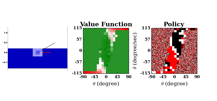
The value function (center), which plots pendulum angular rate against its angle, demonstrates the highly undesirable states of a steeply inclined pendulum (near the horizontal) with high angular velocity in the direction in which it is falling. The policy (right) initially appears random, but converges to the shape shown, with distinct black (counterclockwise torque action) and red (clockwise action) regions in the first and third quadrants respectively, and a white stripe along the major diagonal between. This makes intuitive sense; if the pendulum is left of center and/or moving counterclockwise (third quadrant), for example, a corrective clockwise torque action should certainly be applied. The white stripe in between shows that no torque should be applied to a balanced pendulum with no angular velocity, or if it lies off-center but has angular velocity towards the balance point.

If you pass no command line arguments, no visualization is shown and only the performance graph at the end is produced. For an explanation of each command line argument type:

ipython examples/tutorial/infTrackCartPole_tabular.py -h

When we run the experiment with the tabular representation, we see that the pendulum can be balanced sometimes, but not reliably.

In order to properly assess the quality of the learning algorithm using this representation, we need to average over several independent learning sequences. This means we need to execute the experiment with different seeds.

Running Experiments in Batch

The module Tools.run provides several functions that are helpful for running experiments. The most important one is Tools.run.run().

It allows us to run a specific experimental setup specified by a make_experiment function in a file with multiple seeds in parallel. For details see Tools.run.run().

You find in examples/tutorial/run_infTrackCartPole_batch.py a short script with the following content:

from rlpy.Tools.run import run
run("examples/tutorial/infTrackCartPole_rbfs.py", "./Results/Tutorial/InfTrackCartPole/RBFs",
    ids=range(10), parallelization="joblib")

run("examples/tutorial/infTrackCartPole_tabular.py", "./Results/Tutorial/InfTrackCartPole/Tabular",
    ids=range(10), parallelization="joblib")

This script first runs the infinite track cartpole experiment with radial basis functions ten times with seeds 1 to 10. Subsequently the same is done for the experiment with tabular representation. Since we specified parallelization=joblib, the joblib library is used to run the experiment in parallel on all but one core of your computer. You can execute this script with:

ipython examples/tutorial/run_infTrackCartPole_batch.py

Note

This might take a few minutes depending on your hardware, and you may see minimal output during this time.

Analyzing Results

Running experiments via Tools.run.run() automatically saves the results to the specified path. If we run an Experiments.Experiment instance directly, we can store the results on disc with the Experiments.Experiment.save() method. The outcomes are then stored in the directory that is passed during initialization. The filename has the format XXX-results.json where XXX is the id / seed of the experiment. The results are stored in the JSON format that look for example like:

{"learning_steps": [0, 500, 1000, 1500, 2000, 2500, 3000, 3500, 4000, 4500, 5000],
 "terminated": [1.0, 1.0, 1.0, 1.0, 0.9, 0.8, 0.3, 0.3, 0.0, 0.7, 0.0],
 "return": [-1.0, -1.0, -1.0, -1.0, -0.9, -0.8, -0.3, -0.3, 0.0, -0.7, 0.0],
 "learning_time": [0, 0.31999999999999995, 0.6799999999999998, 1.0099999999999998, 1.5599999999999996, 2.0300000000000002, 2.5300000000000002, 2.95, 3.3699999999999983, 3.7399999999999993, 4.11],
 "num_features": [400, 400, 400, 400, 400, 400, 400, 400, 400, 400, 400],
 "learning_episode": [0, 45, 71, 85, 99, 104, 110, 121, 136, 144, 152],
 "discounted_return": [-0.6646429809896579, -0.529605466143065, -0.09102296558580342, -0.2085618862726307, -0.012117452394591856, -0.02237266958836346, -0.012851215851463843, -0.0026252190655709274, 0.0, -0.0647935684347749, 0.0],
 "seed": 1,
 "steps": [9.0, 14.1, 116.2, 49.3, 355.5, 524.2, 807.1, 822.4, 1000.0, 481.0, 1000.0]}

The measurements of each assessment of the learned policy is stored sequentially under the corresponding name. The module Tools.results provides a library of functions and classes that simplify the analysis and visualization of results. See the the api documentation for details.

To see the different effect of RBFs and tabular representation on the performance of the algorithm, we will plot their average return for each policy assessment. The script saved in examples/tutorial/plot_result.py shows us how:

import rlpy.Tools.results as rt

paths = {"RBFs": "./Results/Tutorial/InfTrackCartPole/RBFs",
         "Tabular": "./Results/Tutorial/InfTrackCartPole/Tabular"}

merger = rt.MultiExperimentResults(paths)
fig = merger.plot_avg_sem("learning_steps", "return")
rt.save_figure(fig, "./Results/Tutorial/plot.pdf")

First, we specify the results we specify the directories where the results are stored and give them a label, here RBFs and Tabular. Then we create an instance of Tools.results.MultiExperimentResults which loads all corresponding results an let us analyze and transform them. In line 7, we plot the average return of each method over the number learning steps done so far. Finally, the plot is saved in ./Results/Tutorial/plot.pdf in the lossless pdf format. When we run the script, we get the following plot

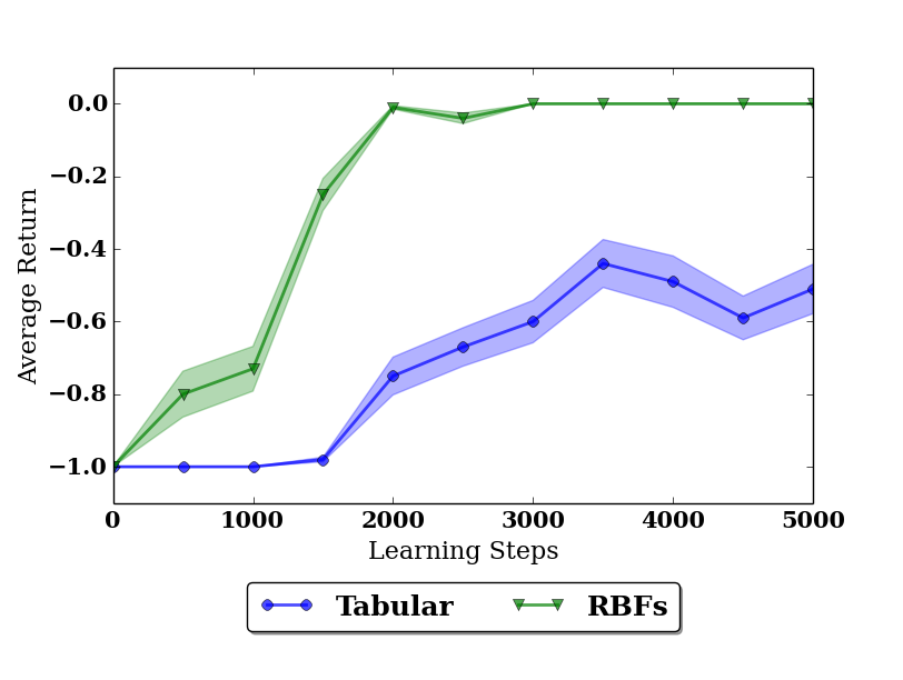
The shaded areas in the plot indicate the standard error of the sampling mean. We see that with radial basis functions the agent is able to perform perfectly after 2000 learning steps, but with the tabular representation, it stays at a level of -0.4 return per episode. Since the value function only matters around the center (zero angle, zero velocity), radial basis functions can capture the necessary form there much more easily and therefore speed up the learning process.

Tuning Hyperparameters

The behavior of each component of an agent can be drastically modified by its parameters (or hyperparameters, in contrast to the parameters of the value function that are learned). The module Tools.hypersearch provides tools for optimizing these parameters to get the best out of the algorithms.

We first need to specify what the hyperparameters for a specific experimental setup are and what values they can possibly take. We therefore again look at part of examples/tutorial/infTrackCartPole_rbfs.py

param_space = {
    "num_rbfs": hp.qloguniform("num_rbfs", np.log(1e1), np.log(1e4), 1),
    'resolution': hp.quniform("resolution", 3, 30, 1),
    'lambda_': hp.uniform("lambda_", 0., 1.),
    'boyan_N0': hp.loguniform("boyan_N0", np.log(1e1), np.log(1e5)),
    'initial_learn_rate': hp.loguniform("initial_learn_rate", np.log(5e-2), np.log(1))}


def make_experiment(
        exp_id=1, path="./Results/Temp/{domain}/{agent}/{representation}/",
        boyan_N0=753,
        initial_learn_rate=.7,
        resolution=25.,
        num_rbfs=206.,
        lambda_=0.75):
    opt = {}
    opt["exp_id"] = exp_id
    opt["path"] = path
    opt["max_steps"] = 5000

The variable param_space contains the definition of the space of hyperparameters we are considering. As the make_experiment function, the variable needs to have exactly this name. For details on how this definition has to look like we refer to the documentation of hyperopt, the package we are using for optimizing hyperparameters.

For each hyperparameter (in this example num_rbfs, resolution, lambda_, boyan_N0 and initial_alpha), the make_experiment function has to have an optional argument with the same name.

The script saved in examples/tutorial/run_parametersearch.py shows us how to perform a quick search good parameters

from rlpy.Tools.hypersearch import find_hyperparameters
best, trials = find_hyperparameters(
    "examples/tutorial/infTrackCartPole_rbfs.py",
    "./Results/Tutorial/InfTrackCartPole/RBFs_hypersearch",
    max_evals=10, parallelization="joblib",
    trials_per_point=5)
print best

Warning

Running this script might take a while (approx. 5-30 min)

The Tools.hypersearch.find_hyperparameters() function is the most important tools for finding good parameters. For details on how to use it see its api documentation.

During the optimization, the results of several an entire experimental run need to be compressed into one target value. The parameter objective controls which quantity to optimize. In this example, it is maximize the reward. We could just take the return of the policy assessment with the most observations (the final policy). However, this can lead to artifacts and causes all hyperparameters that yield the same final performance to be considered equally good, no matter how fast they reach this performance. Therefore, the target value is computed as described below.

The target value is the weighted average over all measurements of the desired quantity (e.g., the average return during each policy assessment). The weights increase quadratically with the observation number, i.e., the return achieved in the first policy assessment has weight 1, the second weight 2, 9, 16, ... This weighting scheme ensures makes the final performance most important but also takes into account previous ones and therefore makes sure that the convergence speed is reflected in the optimized value. This weighting scheme has shown to be very robust in practice.

When we run the search, we obtain the following result:

{‘initial_alpha’: 0.3414408997566183,

‘resolution’: 21.0, ‘num_rbfs’: 6988.0, ‘lambda_’: 0.38802888678400627, ‘boyan_N0’: 5781.602341902433}

Note

This parameters are not optimal. To obtain better ones, the number of evaluations need to be increased to 50 - 100. Also, trials_per_point=10 makes the search more reliable. Be aware that 100 evaluations with 10 trials each result in 1000 experiment runs, which can take a very long time.

We can for example save these values by setting the default values in make_experiment accordingly.

What to do next?

In this introduction, we have seen how to

• run a single experiment with visualizations for getting an intuition of a domain and an agent
• run experiments in batch in parallel on multiple cores
• analyze and create plot the results of experiments
• optimize hyperparameters.

We covered the basic tasks of working with rlpy. You can see more examples of experiments in the examples directory. If you want to implement a new algorithm or problem, have a look at the api documentation. Contributions to rlpy of each flavor are always welcome!

Staying Connected

Feel free to join the rlpy list, rlpy@mit.edu by clicking here. This list is intended for open discussion about questions, potential improvements, etc.

The only real mistake is the one from which we learn nothing.

—John Powell